A formula is an expression which calculates the value of a cell. Functions are predefined formulas and are already available in Excel.
For example, cell A3 below contains a formula which adds the value of cell A2 to the value of cell A1.

For example, cell A3 below contains the SUM function which calculates the sum of the range A1:A2.

To let Excel know that you want to enter a formula, type an equal sign (=).
Operator Precedence
Excel uses a default order in which calculations occur. If a part of the formula is in parentheses, that part will be calculated first. It then performs multiplication or division calculations. Once this is complete, Excel will add and subtract the remainder of your formula. See the example below.
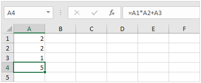
First, Excel performs multiplication (A1 * A2). Next, Excel adds the value of cell A3 to this result.
Another example,
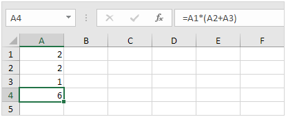
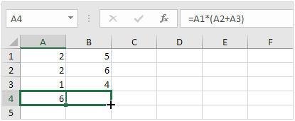
First, Excel calculates the part in parentheses (A2+A3). Next, it multiplies this result by the value of cell A1.
Copy/Paste a Formula
When you copy a formula, Excel automatically adjusts the cell references for each new cell the formula is copied to. To understand this, execute the following steps.
- Enter the formula shown below into cell A4.

2a. Select cell A4, right click, and then click Copy (or press CTRL + c)...
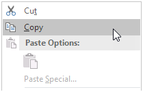
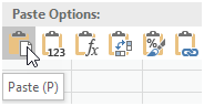
...next, select cell B4, right click, and then click Paste under 'Paste Options:' (or press CTRL + v).
2b. You can also drag the formula to cell B4. Select cell A4, click on the lower right corner of cell A4 and drag it across to cell B4. This is much easier and gives the exact same result!
Result. The formula in cell B4 references the values in column B

Insert a Function
Every function has the same structure. For example, SUM(A1:A4). The name of this function is SUM. The part between the brackets (arguments) means we give Excel the range A1:A4 as input. This function adds the values in cells A1, A2, A3 and A4. It's not easy to remember which function and which arguments to use for each task. Fortunately, the Insert Function feature in Excel helps you with this.
To insert a function, execute the following steps.
1. Select a cell.
2. Click the Insert Function button.
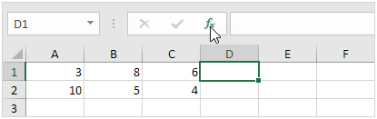
The 'Insert Function' dialog box appears.
3. Search for a function or select a function from a category. For example, choose COUNTIF from the Statistical category.

4. Click OK.
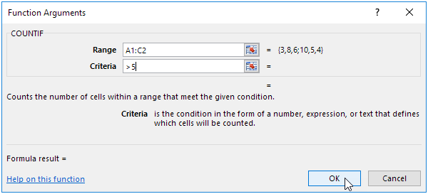
The 'Function Arguments' dialog box appears.
5. Click in the Range box and select the range A1:C2.
6. Click in the Criteria box and type >5.
7. Click OK.
Result. The COUNTIF function counts the number of cells that are greater than 5.
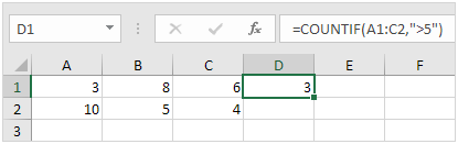
Note: instead of using the Insert Function feature, simply type =COUNTIF(A1:C2,">5"). When you arrive at: =COUNTIF( instead of typing A1:C2, simply select the range A1:C2.
There's no SUBTRACT function in Excel. However, there are several ways to subtract numbers in Excel. Are you ready to improve your Excel skills?
- For example, the formula below subtracts numbers in a cell. Simply use the minus sign (-). Don't forget, always start a formula with an equal sign (=).
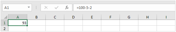
. The formula below subtracts the value in cell A2 and the value in cell A3 from the value in cell A1.

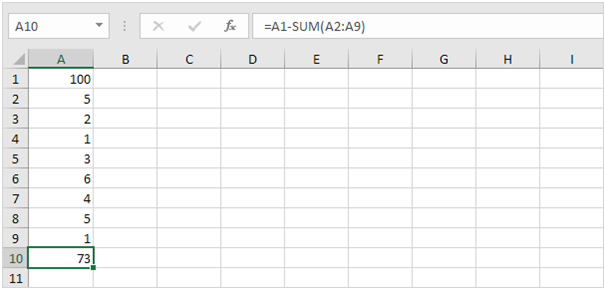
- As you can imagine, this formula can get quite long. Simply use the SUM function to shorten your formula. For example, the formula below subtracts the values in the range A2:A9 from the value in cell A1.
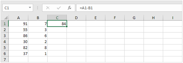
Take a look at the screenshot below. To subtract the numbers in column B from the numbers in column A, execute the following steps.
4a. First, subtract the value in cell B1 from the value in cell A1.
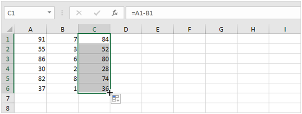
4b. Next, select cell C1, click on the lower right corner of cell C1 and drag it down to cell C6.
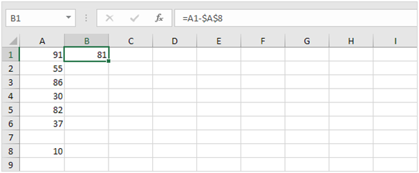
Take a look at the screenshot below. To subtract a number from a range of cells, execute the following steps.
5a. First, subtract the value in cell A8 from the value in cell A1. Fix the reference to cell A8 by placing a $ symbol in front of the column letter and row number ($A$8).
5b. Next, select cell B1, click on the lower right corner of cell B1 and drag it down to cell B6.
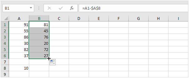
Explanation: when we drag the formula down, the absolute reference ($A$8) stays the same, while the relative reference (A1) changes to A2, A3, A4, etc. Maybe this is one step too far for you at this stage, but it shows you one of the many other powerful features Excel has to offer.
To multiply numbers in Excel, use the asterisk symbol (*) or the PRODUCT function. Learn how to multiply columns and how to multiply a column by a constant.
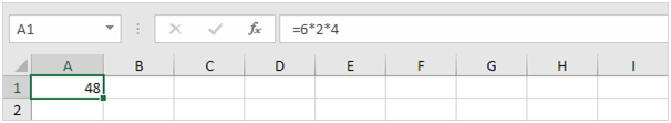
- The formula below multiplies numbers in a cell. Simply use the asterisk symbol (*) as the multiplication operator. Don't forget, always start a formula with an equal sign (=).
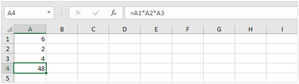
- The formula below multiplies the values in cells A1, A2 and A3.
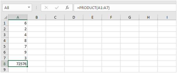
- As you can imagine, this formula can get quite long. Use the PRODUCT function to shorten your formula. For example, the PRODUCT function below multiplies the values in the range A1:A7.
- Here's another example.

Explanation: =A1*A2*A3*A4*A5*A6*A7*B1*B2*B3*B4*C1*8 produces the exact same result.
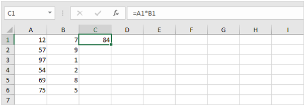
Take a look at the screenshot below. To multiply two columns, execute the following steps.
5a. First, multiply the value in cell A1 by the value in cell B1.
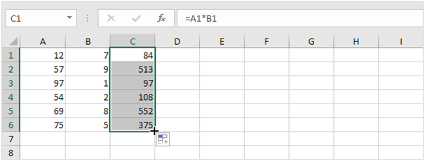
5b. Next, select cell C1, click on the lower right corner of cell C1 and drag it down to cell C6.
Take a look at the screenshot below. To multiply a column of numbers by a constant number, execute the following steps.
6a. First, multiply the value in cell A1 by the value in cell A8. Fix the reference to cell A8 by placing a $ symbol in front of the column letter and row number ($A$8).

6b. Next, select cell B1, click on the lower right corner of cell B1 and drag it down to cell B6.
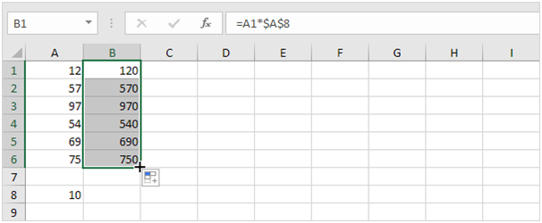
Explanation: when we drag the formula down, the absolute reference ($A$8) stays the same, while the relative reference (A1) changes to A2, A3, A4, etc. You can also use Paste Special to quickly multiply a range of cells by a constant number.
The square root of a number is a value that, when multiplied by itself, gives the number. The SQRT function in Excel returns the square root of a number.
- First, to square a number, multiply the number by itself. For example, 4 * 4 = 16 or 4^2 = 16.
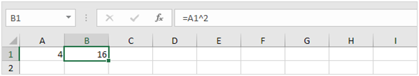
Note: to insert a caret ^ symbol, press SHIFT + 6.
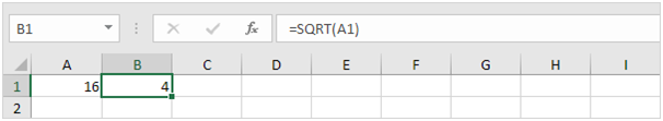
2. The square root of 16 is 4.
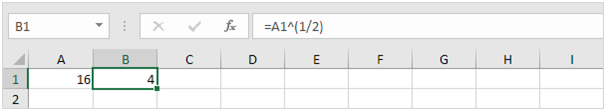
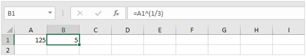
3. Instead of using the SQRT function, you could also use an exponent of 1/2. Don't forget the parentheses.
4. If a number is negative, the SQRT function returns the #NUM! error.
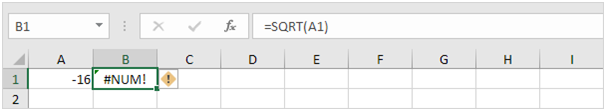
5. You can use the ABS function to remove the minus sign (-) from a negative number.

Excel has no built-in function to calculate the nth root of a number. To calculate the nth root of a number, simply raise that number to the power of 1/n.
6. For example, 5 * 5 * 5 or 5^3 is 5 raised to the third power.

7. The cube root of 125 is 5.
8. For example, 2 * 2 * 2 * 2 * 2 * 2 or 2^6 is 2 raised to the sixth power.
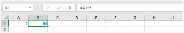
9. The sixth root of 64 is 2.

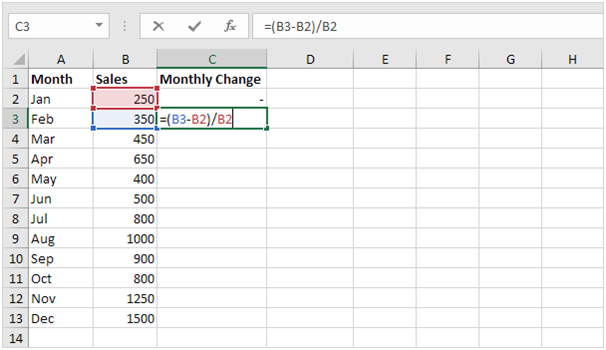
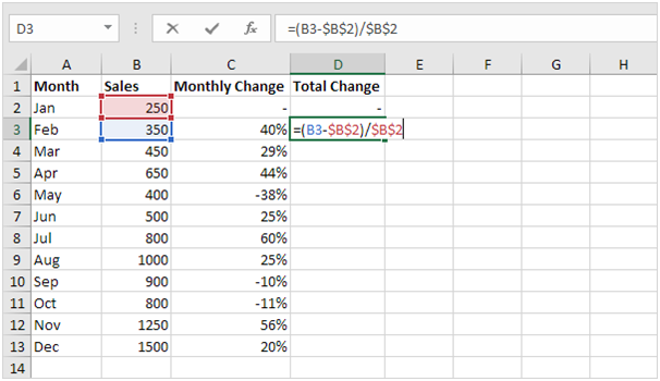
The percent change formula is used very often in Excel. For example, to calculate the Monthly Change and Total Change.
1a. Select cell C3 and enter the formula shown below.
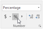
1b. Select cell C3. On the Home tab, in the Number group, apply a Percentage format.

1c. Select cell C3, click on the lower right corner of cell C3 and drag it down to cell C13.
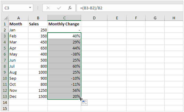
1d. Check if everything went alright.

2a. In a similar way, we can calculate the Total Change. This time we fix the reference to cell B2. Select cell D3 and enter the formula shown below.
2b. Select cell D3. On the Home tab, in the Number group, apply a Percentage format.
2c. Select cell D3, click on the lower right corner of cell D3 and drag it down to cell D13.
2d. Check if everything went alright.
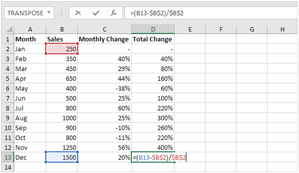
Explanation: when we drag the formula down, the absolute reference ($B$2) stays the same, while the relative reference (B3) changes to B4, B5, B6, etc. Maybe this is one step too far for you at this stage, but it shows you one of the many other powerful features Excel has to offer.
Names in Formulas
Named Range | Named Constant | Name Manager
Create a named range or a named constant and use these names in your formulas. This way you can make your formulas easier to understand.
Named Range
To create a named range, execute the following steps.
- Select the range A1:A4.
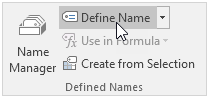
- On the Formulas tab, in the Defined Names group, click Define Name.
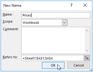
3. Enter a name and click OK.
There's an even quicker way of doing this.
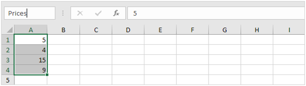
4. Select the range, type the name in the Name box and press Enter.
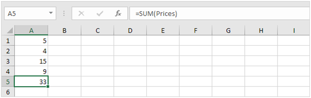
5. Now you can use this named range in your formulas. For example, sum Prices.
Named Constant
To create a named constant, execute the following steps.
- On the Formulas tab, in the Defined Names group, click Define Name.

2. Enter a name, type a value, and click OK.

3. Now you can use this named constant in your formulas.
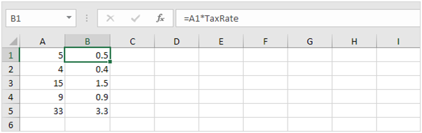
Note: if the tax rate changes, use the Name Manager to edit the name and Excel automatically updates all the formulas that use TaxRate.
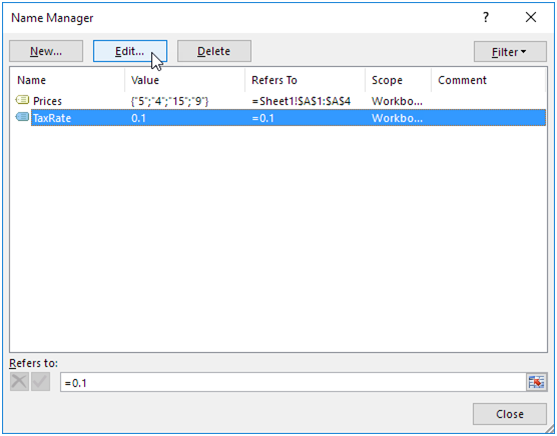
Name Manager
To edit and delete defined names, execute the following steps.
- On the Formulas tab, in the Defined Names group, click Name Manager.

2. For example, select TaxRate and click Edit.
Dynamic Named Range
A dynamic named range expands automatically when you add a value to the range.
1. For example, select the range A1:A4 and name it Prices.
2. Calculate the sum.
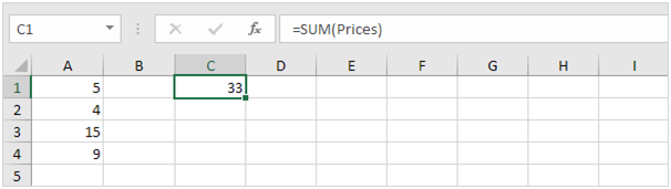
3. When you add a value to the range, Excel does not update the sum.
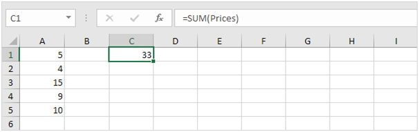
To expand the named range automatically when you add a value to the range, execute the following the following steps.
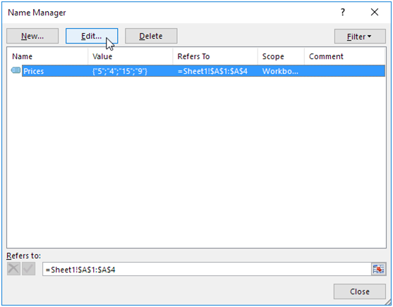
4. On the Formulas tab, in the Defined Names group, click Name Manager.
5. Click Edit.
6. Click in the "Refers to" box and enter the formula =OFFSET($A$1,0,0,COUNTA($A:$A),1)
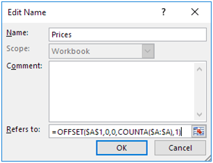
Explanation: the OFFSET function takes 5 arguments. Reference: $A$1, rows to offset: 0, columns to offset: 0, height: COUNTA($A:$A), width: 1. COUNTA($A:$A) counts the number of values in column A that are not empty. When you add a value to the range, COUNTA($A:$A) increases. As a result, the range returned by the OFFSET function expands.
7. Click OK and Close.
8. Now, when you add a value to the range, Excel updates the sum automatically.


Paste Options
Paste | Values | Formulas | Formatting | Paste Special
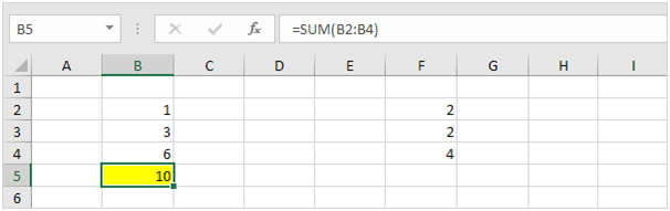
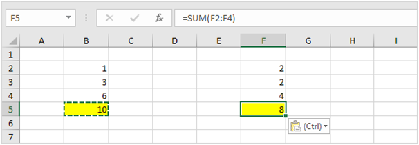
This example illustrates the various paste options in Excel. Cell B5 below contains the SUM function which calculates the sum of the range B2:B4. Furthermore, we changed the background colour of this cell to yellow and added borders.
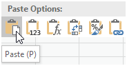
Paste
The Paste option pastes everything.
1. Select cell B5, right click, and then click Copy (or press CTRL + c).
2. Next, select cell F5, right click, and then click Paste under 'Paste Options:' (or press CTRL + v).
Result.
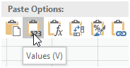
Values
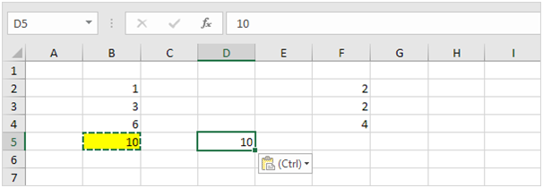
The Values option pastes the result of the formula.
1. Select cell B5, right click, and then click Copy (or press CTRL + c).
2. Next, select cell D5, right click, and then click Values under 'Paste Options:'
Result.
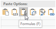
Formulas
The Formulas option only pastes the formula.
1. Select cell B5, right click, and then click Copy (or press CTRL + c).
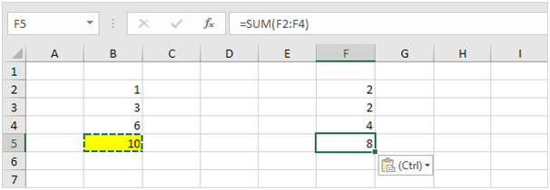
2. Next, select cell F5, right click, and then click Formulas under 'Paste Options:'
Result.
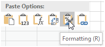
Formatting
The Formatting option only pastes the formatting.
1. Select cell B5, right click, and then click Copy (or press CTRL + c).
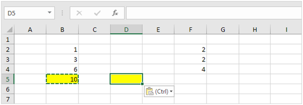
2. Next, select cell D5, right click, and then click Formatting under 'Paste Options:'
Result.
Note: the Format Painter copy/pastes formatting even quicker.
Paste Special
The Paste Special dialog box offers many more paste options. To launch the Paste Special dialog box, execute the following steps.
- Select cell B5, right click, and then click Copy (or press CTRL + c).
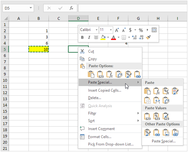
The Paste Special dialog box appears.
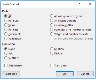
Note: here you can also find the paste options described above. You can also paste comments only, validation criteria only, use the source theme, all except borders, column widths, formulas and number formats, values and number formats. You can also use the Paste Special dialog box to perform quick operations, skip blanks and transpose data.
Status Bar
The quickest way to see the average, count, numerical count, minimum, maximum or sum of selected cells is by taking a look at the status bar.
- Select a range of cells.
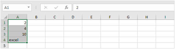
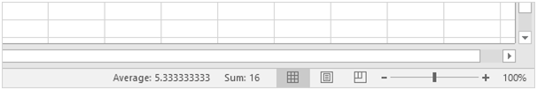
2. Look at the status bar at the bottom of your window to see the sum of these cells.
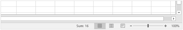
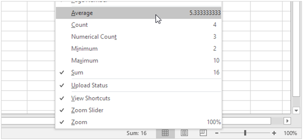
Result:
Quick Operations
Use the 'Paste Special Operations' to quickly perform operations on a range of cells in Excel.
1. Select cell D3.
2. Right click, and then click Copy.
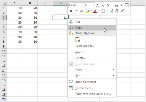
3. Select the range A1:B8.
4. Right click, and then click Paste Special.
5. Click Multiply.
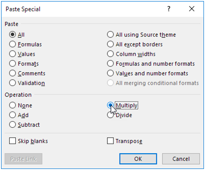
Note: you can also Divide, Add or Subtract a value.
6. Click OK.
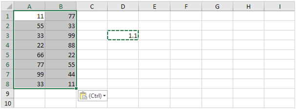
Note: all values are increased by 10 percent. Without this feature, you would have to create a temporary range (with formulas that multiply the values in the range A1:B8 by 1.1) and then replace the range A1:B8 by copy and pasting the temporary range as values.
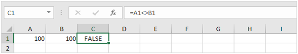
Not Equal To
In Excel, <> means not equal to. The <> operator in Excel checks if two values are not equal to each other. Let's take a look at a few examples.
- The formula in cell C1 below returns TRUE because the text value in cell A1 is not equal to the text value in cell B1.

2. The formula in cell C1 below returns FALSE because the value in cell A1 is equal to the value in cell B1.
3. The IF function below calculates the progress between a start and end value if the end value is not equal to an empty string (""), else it displays an empty string (see row 5).

Note: visit our page about the IF function for more information about this Excel function.
4. The COUNTIF function below counts the number of cells in the range A1:A5 that are not equal to "red".

Note: visit our page about the COUNTIF function for more information about this Excel function.
5. The COUNTIF function below produces the exact same result. The & operator concatenates the 'not equal to' operator and the text value in cell C1.

6. The COUNTIFS function below counts the number of cells in the range A1:A5 that are not equal to "red" and not equal to "blue".

Explanation: the COUNTIFS function in Excel counts cells based on two or more criteria. This COUNTIFS function has 2 range/criteria pairs.
7. The AVERAGEIF function below calculates the average of the values in the range A1:A5 that are not equal to 0.

Note: in other words, the AVERAGEIF function above calculates the average excluding zeros.
Here are some functions that I used quite often.
1) Two functions working together
=IFERROR(VLOOKUP(A2,STOCK,5,FALSE),0)
To explain
IFERROR(...,0) will give you a 0 when an error occurs (ie no match was found), you can use any character if you wish but zero is good for doing math.
VLOOKUP(A2,STOCK,5,FALSE) this will use cell A2 as the key to be found in table "STOCK" (I normally place this on a separate sheet) and will return the 5th cell and FALSE is to have an exact match.
Example table STOCK
|
Stock No. |
Make |
Model |
Engine No. |
Cost |
|
466414 |
AUDI |
A4 B8 |
CG42720 |
68800.00 |
|
469686 |
AUDI |
A4 B8 2.7 |
CG45852 |
63600.00 |
Please ensure that in your table you have no duplicates as VLOOKUP will only find the first occurrence of the value in cell A2
Good practice is to create a pivot table from your data and make that the table you use as this will ensure no duplicates.
2) CONCATENATE
To use these examples in Excel, copy the data in the table below, and paste it in cell A1 of a new worksheet.
|
Data |
||
|
brook trout |
Andreas |
Hauser |
|
species |
Fourth |
Pine |
|
32 |
||
|
Formula |
Description |
|
|
=CONCATENATE("Stream population for ", A2, " ", A3, " is ", A4, "/mile.") |
Creates a sentence by joining the data in column A with other text. The result is Stream population for brook trout species is 32/mile. |
|
|
=CONCATENATE(B2, " ", C2) |
Joins three things: the string in cell B2, a space character, and the value in cell C2. The result is Andreas Hauser. |
|
|
=CONCATENATE(C2, ", ", B2) |
Joins three things: the string in cell C2, a string with a comma and a space character, and the value in cell B2. The result is Andreas, Hauser. |
|
|
=CONCATENATE(B3, " & ", C3) |
Joins three things: the string in cell B3, a string consisting of a space with ampersand and another space, and the value in cell C3. The result is Fourth & Pine. |
|
|
=B3 & " & " & C3 |
Joins the same items as the previous example, but by using the ampersand (&) calculation operator instead of the CONCATENATE function. The result is Fourth & Pine. |
|
Use the ampersand & character instead of the CONCATENATE function. |
The ampersand (&) calculation operator lets you join text items without having to use a function. For example,=A1 & B1 returns the same value as=CONCATENATE(A1,B1). In many cases, using the ampersand operator is quicker and simpler than using CONCATENATE to create strings. |
|
Use the TEXT function to combine and format strings. |
The TEXT function converts a numeric value to text and combines numbers with text or symbols. For example, if cell A1 contains the number 23.5, you can use the following formula to format the number as a dollar amount: =TEXT(A1,"$0.00") Result: $23.50 |
3) LEFT and RIGHT
LEFT returns the first character or characters in a text string, based on the number of characters you specify.
Cell A2 Sale Price
=LEFT(A2,4) First four characters in the Cel A2
Sale
RIGHT returns the last character or characters in a text string, based on the number of characters you specify.
=RIGHT(A2,5) Last 5 characters of the Cel A2
Price
4) TRIM(text)
Removes all spaces from text except for single spaces between words. Use TRIM on text that you have received from another application that may have irregular spacing.
=TRIM(" First Quarter Earnings ")
Removes leading and trailing spaces from the text in the formula (First Quarter Earnings)
5) LEN(text)
LEN returns the number of characters in a text string.
A2 = Phoenix, AZ
=LEN(A2) Length of the first string (11)
6) Dsum function
The Excel Dsum function calculates the sum of a field (column) in a database for selected records, that satisfy user-specified criteria.
The function is very similar to the Excel Sumifs function, which was first introduced in Excel 2007.
The syntax of the Excel Dsum function is:
DSUM( database, field, criteria )
where the arguments are:
database - A range of cells containing the database. The top row of the database should specify the field names.
field -
The field (column) within the database, that is to be summed.
This can either be a field number, or can be the field name (i.e. the header in the top row of the database) encased in quotes (e.g. "Area", "Quarter", etc).
criteria -
A range of cells that contain the criteria, to specify which records should be included in the calculation.
The range can include one or more criteria, which are presented as a field name in one cell and the condition for that field in the cell below.
E.g.
Quarter Area
>2 South
The following examples are based on the simple database (below), which stores the sales figures for four sales representatives, working in the North or South area, over the four quarters of a year.
| A | B | C | D | |
| 1 | Quarter | Area | Sales Rep. | Sales |
| 2 | 1 | North | Jeff | $223,000 |
| 3 | 1 | North | Chris | $125,000 |
| 4 | 1 | South | Carol | $456,000 |
| 5 | 1 | South | Tina | $289,000 |
| 6 | 2 | North | Jeff | $322,000 |
| 7 | 2 | North | Chris | $340,000 |
| 8 | 2 | South | Carol | $198,000 |
| 9 | 2 | South | Tina | $222,000 |
| 10 | 3 | North | Jeff | $310,000 |
| 11 | 3 | North | Chris | $250,000 |
| 12 | 3 | South | Carol | $460,000 |
| 13 | 3 | South | Tina | $395,000 |
| 14 | 4 | North | Jeff | $261,000 |
| 15 | 4 | North | Chris | $389,000 |
| 16 | 4 | South | Carol | $305,000 |
| 17 | 4 | South | Tina | $188,000 |
Example 1
In the example below, the Dsum function is used to calculate the total sales in quarters 3 & 4, in the "North" area. The criteria are specified in cells F1 - G2 and the Dsum formula is shown in cell F3.
F G
1 Quarter Area
2 >2 North
3 =DSUM( A1:D17, "Sales", F1:G2 )
The above Dsum function calculates the sum of the values in cells D10, D11, D14 & D15, and therefore returns the value $1,210,000.
Example 2
In the example below, the Dsum function is used to calculate the total sales in quarter 3, by sales reps with names beginning with the letter "C". Again, the criteria are specified in cells F1 - G2 and the Dsum formula is shown in cell F3.
F G
1 Quarter Sales Rep.
2 3 C*
3 =DSUM( A1:D17, "Sales", F1:G2 )
The above Dsum function sums the values in cells D11 and D12 and so returns the value $710,000.
Note that, in the above two examples, instead of typing in "Sales" for the field argument, we could have simply used the number 4 (to denote the 4th column of the database).
7) Sumifs function
The Excel Sumifs function finds values in one or more supplied arrays, that satisfy a set of criteria, and returns the sum of the corresponding values in a further supplied array.
The function is new in Excel 2007, and so is not available in earlier versions of Excel.
The syntax of the Sumifs function is:
SUMIFS( sum_range, criteria_range1, criteria1, [criteria_range2, criteria2], ... )
Where the function arguments are:
sum_range - An array of numeric values (or a range of cells containing numbers) which are to be added together if the criteria are satisfied.
criteria_range1
[criteria_range2], ... -
Arrays of values (or ranges of cells containing values) to be tested against the respective criteria1, criteria2, ...
(The supplied criteria_range arrays must all have the same length as the sum_range).
criteria1,
[criteria2], ... - The conditions to be tested against the values in criteria_range1, [criteria_range2], ...
Note that:
The Sumifs function can handle up to 127 pairs of criteria_range and criteria arguments.
Each of the supplied criteria can be either:
a numeric value (which may be an integer, decimal, date, time, or logical value) (e.g. 10, 01/01/2008, TRUE)
or
a text string (e.g. "Name", "Thursday"), which can include wildcards
Wildcards
You can use the following wildcards in text-related criteria:
? - matches any single character
* - matches any sequence of characters
Note that, if you actually want to find the ? or * character, type the ~ symbol before this character in your search.
E.g. the condition "a*e" will match all cells containing a text string beginning with "a" and ending in "e".
or
an expression (e.g. ">12", "<>0").
If your criteria is a text string or an expression, this must be supplied to the Sumifs function in quotes;
The Excel Sumifs function is not case-sensitive. So, for example, the text strings "TEXT" and "text" will be considered to be equal.
The following examples are based on the simple database above (in the Dsum function)
Example 1
To find the sum of sales in the North area during quarter 1:
=SUMIFS( D2:D13, A2:A13, 1, B2:B13, "North" )
which gives the result $348,000.
In this example, the Excel Sumifs function identifies rows where:
The value in column A is equal to 1
and
The entry in column B is equal to "North"
and calculates the sum of the corresponding values from column D.
I.e. this formula finds the sum of the values $223,000 and $125,000 (from cells D2 and D3).
Example 2
Again, using the data spreadsheet above, we can also use the Sumifs function to find the total sales for "Jeff", during quarters 3 and 4:
=SUMIFS( D2:D13, A2:A13, ">2", C2:C13, "Jeff" )
This formula returns the result $571,000.
In this example, the Excel Sumifs function identifies rows where:
The value in column A is greater than 2
and
The entry in column C is equal to "Jeff"
and calculates the sum of the corresponding values in column D.
I.e. this formula finds the sum of the values $310,000 and $261,000 (from cells D8 and D11).
- You are here:
-
Home

- Excel Tutorial